1. 1.Sample Test
   

    1.1 z－test

     两个样本方差已知，且相等

     z= (xbar-ybar)   / (sigma*sqrt(1/m +1/n) )

    1.2 t-test, F-test

    在sigma未知的情况下

    单样本，可以检验mu（平均值）取值

    双样本，可以比较检验两个样本间平均值的关系

    t.test(  )

    中间有很多参数可以设置，包括是否pair, Variance是否equal, Alternative Hypothesis 是什么。

     用Ftest检验方差是否相等

1. *Special case
   

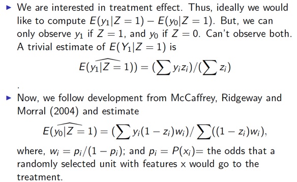
In Practice Observational samples 在实际的观测样本中，对比实验组和观测组下结论之前，除了用回归的方式排除其他因素干扰，亦可选用Propensity Score Methods

第一步，用逻辑斯特回归计算Propensity Score

第二步：方法一，选用相近的score作为matching pair

               方法二，将Propensity score转换为odds, 作为weights。进行比较。

具体操作参见以下codes：

//

//  lalonde_PropensityScoreExample.r

// 

//

//  Created by Siddhartha Dalal on 4/15/14.

//The example uses the LaLonde (1986) experimental data which is based on a nationwide job training experiment. The observations are individuals, and the outcome of interest is real earnings in 1978. There are eight baseline variables age (age), years of education (educ), real earnings in 1974 (re74), real earnings in 1975 (re75) and in 78 (re78), and a series of indicator variables. The indicator variables are black (black), Hispanic (hisp), married (married) and lack of a high school diploma (nodegr).

//

require(Matching)

data(lalonde)

#attach(lalonde) #data from library Matching - lalonde

par(ask=T)

for (i in 1:length(names(lalonde))) {hist(lalonde[[i]],xlab=names(lalonde[i]),main= names(lalonde[i]))}        ## 不同变量是否接受了treatment的柱状图

Tr <- lalonde$treat

#Propensity Score computation

glm1 <- glm(Tr ~ age + educ + black + hisp + married + nodegr +

+ re74 + re75, family = binomial, data = lalonde)

plot(ecdf(glm1$fit))

propscore=glm1$fitted/(1-glm1$fitted)

plot(ecdf(propscore))

#Estimation of Average Effect for Treated Population (ATT)

before_after_prop=function(comp_var,propscore,Tr,plt=FALSE){

#given comparison variable where you want to measure balance, and corresponding propscore as well as indicator for treatment variable, compute means before adjustment and after, also compute ATT

y1=comp_var[Tr==1]     ##comp_var是目标数值

y0=cbind(comp_var,propscore)[Tr==0,]

meany1_tr=mean(y1)

meany0_ntr=mean(y0[,1])

meany0_tr=weighted.mean(y0[,1],y0[,2])

meany1_ntr=weighted.mean(y1,1/propscore[Tr==1])

print(c("actually","mean if not treated","mean if treated"))

print(c("treated",meany1_ntr,meany1_tr))

print(c("controlled",meany0_ntr,meany0_tr))

ATT=meany1_tr-meany0_tr #ATT=Average Treatment for Treated for the covariate-i.e. it is mean of the discrepancy between before and after matching

ATT.w=meany1_tr-meany0_ntr #without propensity score matching

##See how well is the samples balanced

if (balance==TRUE) {py1<-propscore[Tr==1]; py0<-propscore[Tr==0]

par(mfrow=c(2,1))

hist(py1); hist(py0)

#Permutation test

x<-as.list(seq(range(propscore)[1],range(propscore)[2],by=0.001))

Fx1<-sapply(x,function(x) sum(as.numeric(py1<=x))/length(py1))

Fx2<-sapply(x,function(x) sum(as.numeric(py0<=x))/length(py0))

t<-which(Fx2!=0 & Fx2!=1)

ad2.obs<-sum((Fx1[t]-Fx2[t])^2/(Fx2[t]*(1-Fx2[t])))

} else {}

return(list(mean_tr_tr=meany1_tr,mean_tr_ntr=meany0_tr,mean_ntr=meany0_ntr,ATT=ATT,ATT.w=ATT.w, balance.statistic=ad2.obs))

}

#The following variables were matched. Let us see balance on it after adjustment

before_after_prop(lalonde$nodegr,propscore,Tr)  

before_after_prop(lalonde$hisp,propscore,Tr)

before_after_prop(lalonde$re75,propscore,Tr)

#The following varialble is outcome varaible, let us see the performance on it

before_after_prop(lalonde$re78,propscore,Tr, balance=TRUE)

2. Linear Regression

    2.1 t-test

    回归出来的模型summary(fit)，在coefficient跟着的t值,服从 t 分布，df＝n－p

    confint(fit, level=)

    置信区间

    2.2 General linear test (F-test)

    利用anova表格，F-stat＝（SSE(R) - SSE(F) )/ (dfr -dff)  / MSE(F)  ~F(dfr-dff, dff)

    anova(fit)

3. General Linear Regression

    3.1 Wald Test

    回归出来的模型summary(fit)，在coefficient后跟着的Z－score， 服从正太分布

    3.2 Drop-in Deviance Test

    同样在summary(fit)中关注Residual Deviance， 越小越好

    Difference in Deviance~ Chisq with df= difference in df

    3.3 The likelihood Ratio Test